
Hyperspectral imaging has grown increasingly popular over the past ten years in military, industrial, and scientific arenas. The ability to precisely characterize the color of a viewed item, whether a camouflaged vehicle, a bruise on an arm or on fruit, or a wide swath of vegetation, allows the user to make informed decisions only dreamed of in the past. What once required large, delicate, and expensive laboratory spectrometers is now being done in real time aboard satellites, unmanned aerial vehicles, and portable handheld units.
Background and Progress
Expanding a vision system to create many more “bins” can be exceptionally complicated. In 1999, Deposition Sciences, Inc. (DSI) was contracted to coat a series of 16 beamsplitters. These beamsplitters were configured in four primary optical chains, each with four secondary chains, resulting in sixteen discrete optical paths, each terminating at a separate detector. The end result was a sixteen-channel spectral imaging system covering a wavelength range from 400 - 900 nm. Each optical element had to maintain a transmittance and reflectance of greater than 98% to ensure a final signal level at the detectors of at least 90%. While this system worked as designed, it was large, expensive, and delicate. It was suitable for the benchtop demonstration required, but not for many of the in-field applications needed by today’s sensor systems.
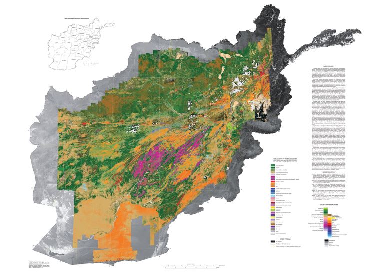
Compare that system with the hyperspectral data collected by the USGS in Afghanistan in 20071. Using an airborne HyMap system from HyVista Corporation , the USG Survey generated detailed maps of the surface mineral distribution across approximately 440,000 km2 (172,000 mi2). Thirty-one different classes of materials were identified and mapped in this survey. A subset of the results is shown in Figure 1. These data were collected over a series of 28 flights, using four different modules in one instrument to cover a spectral range of 0.43 to 2.48 microns. Images were processed over 128 color bands, each 14-20 nm wide. Full details of the survey, including a discussion of the methodology, can be found at the USGS website .
Enabling Technologies
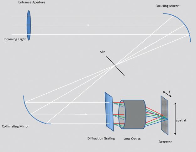
There are two broadly defined areas of technology which have enabled the development and advancement of hyperspectral imaging. They are the development of inexpensive, high quality diffraction gratings and the advancements in multiple dimension data processing. In order to see how these technologies have improved the state of hyperspectral imaging, it is necessary to take a brief look at how most current systems operate. Note that this is a general discussion. Most of the companies offering instruments or services have unique, proprietary approaches that distinguish one from the other. We will only look at a simplified system that identifies some of the key features. Such a simplified system is shown in Figure 2.
Most hyperspectral imaging systems consist of imaging optics, a narrow slit, a diffraction grating, and a 2-dimensional focal plane array (FPA) detector (usually CCD or CMOS). The image is projected through the slit onto the diffraction grating where the light is split into discrete wavelengths and physically separated before being projected onto the focal plane array. One dimension of the FPA corresponds to the wavelength of light, as separated by the diffraction grating. The other dimension corresponds to the “vertical” position along the slit.
At each X-Y coordinate, a pixel is energized to some level, based on the intensity of the light at that position and wavelength. What results is a 3-dimensional array (position on slit, wavelength and intensity) for each narrow slit width. By indexing the slit width, one can map the entire image into a 4-dimensional array. This indexing (called “pushbrooming”) can be done by moving the slit, or by moving the sensor device. In the case of the USGS survey of Afghanistan, cited above, each slit width corresponded to a single flight line, or pass of the airplane. Determining how much overlap to use, as well as what known standards or features to use for calibration, is critical in getting reliable data.
The second piece of the hyperspectral imaging puzzle is the vast improvement in high-speed computer data analysis. Virtually every system vendor has a readymade software package that ties in GPS coordinates, interleaves the pushbroom data (properly accounting for the overlap), automatically checks against known features and is able to operate at cycles in excess of 500 frames per second (fps). This capability is absolutely crucial for making the jump from processing a single line of data to processing an entire composite image.The USGS work cited above produced over 800 million pixels of data.
Current State of the Art
Many vendors surveyed for this article produce systems with at least 100 bands for the spectral range, with full width at half maximum (FWHM) bandwidths on the order of 1 - 5 nm. Frame capture rates run from 100 - 600 fps. Of course actual performance is highly dependent on the system configuration parameters such as the characteristics of the diffraction grating, the field of view, and the type of sensor used. IR sensors generally must be cooled, adding to the size and weight of the device.
In fifteen short years, the industry has made great strides in hyperspectral imaging. Areas such as agriculture, natural resource and the biological sciences have led the way. Law enforcement, aerospace, and defense can tap into this reservoir of knowledge to define and acquire hyperspectral imaging systems virtually off the shelf. In addition to the resources cited in this article, the Hyperspectral Imaging Foundation , founded in 2012, is an excellent repository of information and platform for discussion.
This article was written by Kevin P. Gibbons, Program Manager, Government Products Group, Deposition Sciences, Inc. (DSI®) (Santa Rosa, CA). For more information, contact Mr. Gibbons at
References
- Kokaly, R.F., King, T.V.V., Hoefen, T.M., Dudek, K.B., and Livo, K.E., 2011, Surface materials map of Afghanistan: carbonates, phyllosilicates, sulfates, altered minerals, and other materials: U.S. Geological Survey Scientific Investigations Map 3152–A, one sheet, scale 1:1,100,000. Also available at http://pubs.usgs.gov/sim/3152/A/
- Norak Electro Optik, Solheimsveien 62A, N-1473 Lorenskog, Norway; http://www.hyspex.no